Lloyd Allison, www.allisons.org/ll/MML/, May 2014,
Faculty of Information Technology, Clayton Campus, Monash University, Australia

#2014/277

Abstract: This report concerns the information content of a graph, optionally conditional on one or more background, "common knowledge" graphs. It describes an algorithm to estimate this information content, and includes some examples based on chemical compounds.

Keywords: Graph, network, complexity, information content, sex drugs, rock and roll (not).

Also see LaTex/pdf version [arxiv.org/abs/2008.04744]['20].

Introduction

The information content of a graph, in bits, equals the minimum length of a message [WB69], in an efficient code, that sends the graph from a transmitter to a receiver -- the optimal compressed size of the graph. If, as is very often the case, the "true" statistical model describing the population of graphs is unknown, information content can be estimated by using a plausible model.

Some literature on graphs uses 'compression' in a different sense, for example, "a ‘compression’ G* of a graph G ... (a) G* is a graph with m* edges, where m* < # edges in G, (b) it is comp. easy to convert G into G* and v.v." [FM95,p.1]. (Note, G* likely has more Vertices than G.) Such G and G* contain exactly the same information because it is "easy to convert" one into the other and back again, so this is not compression in the usual data compression sense. However, G* might be easier, in the sense of more convenient, to compress well, if not optimally, compared to G. And, being sparser, G* might also appear subjectively simpler, particularly when drawn in 2D.

The following sections discuss various issues to do with graphs and their representations, a prototype algorithm, and an application to the structures of chemical compounds.

Graphs

A graph, G=⟨V,E⟩, can be directed or undirected. Each Edge is optionally labelled with a value of type et. Each Vertex is optionally labelled with a value of type vt. If Vertices are unlabelled, set et=( ), the trivial type, and if Edges are unlabelled, set vt=( ).

Depending on the application:

Vertices may or may not be labelled, and

Edges may or may not be labelled.

 

Graph no (v,v) (v,v) allowed undirected |V|×(|V|-1)/2 |V|×(|V|+1)/2 directed |V|×(|V|-1) |V|2     max. number of Edges

 

Unless otherwise specified, the following are not allowed here:

self-loops, ⟨v, v⟩, and

multiple Edges, ⟨u,v⟩₁, ⟨u,v⟩₂, ..., i.e., multi-graphs.

Vertex orderings

To encode a graph, one encodes some representation of the graph, notably the adjacency matrix or the adjacency lists representations. Since every non-redundant representation contains the same information, that is the graph, an optimal encoding of any representation must give the same minimum message length (MML) as any other. However one representation might be easier - more convenient - to compress than another.

A representation may contain more information than just the graph, in particular it may imply a certain distinguishable ordering of the Vertices. There are |V|! possible orderings of the Vertices although not all are necessarily distinguishable. A Vertex ordering (numbering) is arbitrary -- changing it does not change the graph -- such a representation contains log₂(|V|! / |A|) bits of information over and above the graph itself, where A is the automorphism group of G [Sta05]; the appendix contains examples. (Note that |A|=1 if every Vertex has a unique label.)

An adjacency matrix representation of a graph implies a particular ordering of the Vertices. Any distinguishable ordering could be used, each corresponding to a different adjacency matrix. Alternatively, some canonical ordering [various₀], and adjacency matrix, could be used, for example, the one with its rows in lexicographically non-descending order. An optimal encoding of it must somehow take advantage of that property. Alternatively, to calculate the information content of the graph, encode any adjacency matrix and subtract log₂(|V|! / |A|) bits.

Adjacency matrix

An adjacency matrix of a graph can be trivially encoded using 1 bit per possible Edge. This is only optimal if half of the possible Edges exist, and the existence of an Edge is independent of other Edges, and of labels if present.

When the Edge density is not known apriori, the very least that should be done is to model the entries of the adjacency matrix by a binomial distribution. This is optimal if the existence of an Edge is independent of other Edges. The hypothesis has one parameter, the expected Edge density, which is the same in all parts of the graph. This does not mean that all Vertices have the same degree. Note, subtly different is the hypothesis that the Edge density is homogeneous (and we do not care what the density is) which can be realised by using the adaptive coding of binomial data and which saves a fraction of a bit in total.

For a directed graph, if it is believed that the degrees of Vertices may differ and are independent, and the existence of Edges are independent, an approriate model is to use one binomial distribution per row (or column) of the adjacency matrix. The model has one parameter per Vertex, being the out- (or in-) Edge density of the Vertex. (Many simple variations are possible, for example, a model could have two density parameters, for "low" and "high" degree vertices, plus a binomial distribution over into which of these "classes" Vertices fall.)

The situation is more complicated for an undirected graph where an adjacency matrix is necessarily symmetric (equivalently upper or lower triangular). The existence of an undirected Edge (u,v) depends on the neighbourliness of both u and v. These cannot be independent: consider "u is adjacant to all, and v is adjacent to none." It is tempting to average the contributions of u and v.

Adjacency lists

An adjacency-lists representation of a graph contains the same information as an adjacency matrix so, if optimally encoded, they must have the same length. It takes log₂|V| bits to specify a given Vertex in some ordering. The adjacency list, L, of some Vertex does not contain the Vertex and contains no Vertex twice, so it might as well be sorted ascending, say (otherwise it contains log₂|L| bits of extra, non-graph information). The information content if L is info(|L|) + log₂(|V|-1) + ... log₂(|V|-|L|) - log₂(|L|!) bits. The distribution on |L| models the Edge density of the graph.

For comparison, the information in one row of the adjacency matrix (see above), using the adaptive coding for a binomial distribution and assuming a uniform prior on the number of 1s is [WB69]: log₂(|V|!) - log₂((#1)!) - log₂((#0)!), where #1 + #0 = V - 1. Now, log |V| is info(|L|). log₂((|V|-1)!) - log₂((#0)!) = log₂((|V|-1)!) - log₂(|V|-1-|L|) = log₂(|V|-1) + ... log₂(|V|-|L|). And - log₂((#1)!) = - log₂(|L|!). So, the information content of the adjacency list of a Vertex in the adjacency lists representation, and of the corresponding row in the adjacency matrix representation, are equal, as they should be.

Special classes of graph

Methods have been devised to efficiently encode some special classes of graph:

rooted strict binary tree, about 1-bit per Vertex [various₁],

rooted general tree, about 2 bits per Edge [various₂],

plane graph, about 4 bits per Edge [Tur84], later log₂(14) bits per Edge [Via08].

The above examples rely on global properties of a graph and do not attempt to take advantage of any kind of repeated pattern.

More interesting are attempts to base graph compression on recognising patterns (motifs), that are repeated, possibly approximately, that is with variations. This is particularly so where a graph has semantics - where its structure carries meaning.

A prototype algorithm

The idea is to extend the Lempel-Ziv style of sequence compression to graphs: traverse the graph in some arbitrary order. At each step in the traversal there is the next element, the next unknown - a Vertex or an Edge. Seek scored matches to the recently traversed, and hence known, context in the common knowledge, on the basis that what happened "then" might happen "now". Form a probability distribution over the possible values for the next element (Vertex (label, arity), Edge (label, looping)) using the scored (weighted) matches. The common knowledge consists of zero or more given graphs. (For simplicity, the prototype does not search for matches to the context within the traversed part of the graph being compressed, but this is clearly possible in principle.)

The method described below calculates the information content of an undirected graph. It is clear that, in principle, a "similar method" can be devised for directed graphs. (The probability distribution calculated at each step could be used, with an arithmetic compressor, say, to perform actual data compression.)

The prototype does not attempt to "recover" the extra information from the arbitrary Vertex ordering (see automorphism group earlier).

It is sufficient to consider a single connected component; a disconnected graph can be treated one component at a time, including earlier components in the common knowledge, if desired.

data Vertex vt et = Vertex vt Int [Edge vt et]

data Edge vt et = Edge et (Vertex vt et) (Vertex vt et)

-- a Vertex contains an arbitrary but unique Int, only to identify it; this is not a "label".

-- e.g., ...
data Entity     = Utility | House  deriving (Eq, Enum, Bounded, Show, Read)
data Connection = Elec | Gas | H2O deriving (Eq, Enum, Bounded, Show, Read)

k33 = v00 where                  -- complete, bipartite, labelled
  v00 = Vertex Utility 0
        [Edge Elec v00 v10, Edge Elec v00 v11, Edge Elec v00 v12]
  v01 = Vertex Utility 1
        [Edge Gas v01 v10, Edge Gas v01 v11, Edge Gas v01 v12]
  v02 = Vertex Utility 2
        [Edge H2O v02 v10, Edge H2O v02 v11, Edge H2O v02 v12]

  v10 = Vertex House 3
        [Edge Elec v10 v00, Edge Gas v10 v01, Edge H2O v10 v02]
  v11 = Vertex House 4
        [Edge Elec v11 v00, Edge Gas v11 v01, Edge H2O v11 v02]
  v12 = Vertex House 5
        [Edge Elec v12 v00, Edge Gas v12 v01, Edge H2O v12 v02]

Traversal of an undirected graph

An undirected graph is represented by an adjacency-lists data structure; if Vertices u and v are adjacent, the data structure links u to v and also links v to u.

The information-content calculations rely on a graph traversal. The traversal arrives at a Vertex via an incoming Edge and follows an Edge out from a Vertex, so the immediate context of an Edge is a Vertex, and the immediate context of a Vertex is an Edge (except for the initial Vertex which has the empty context).

traverse_undirected fv fe v =
  ...

Traverse a graph accessible from Vertex v, apply fv to each Vertex and fe to each Edge, and return a list of type [Either fv_result fe_result]. The output contains one element per Vertex and one element per Edge.

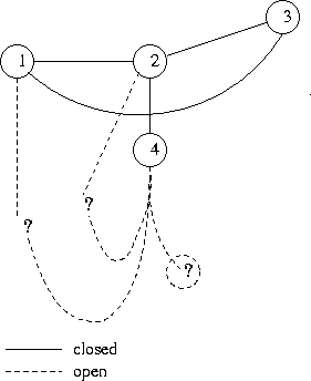
During traversal, a Vertex has a 'status', one of UNVISITED | VISITING | VISITED (see figure 1). Initially every Vertex is UNVISITED. A Vertex becomes VISITING when the traversal first accesses it, and remains so while any of its Edges are yet to be traversed. A Vertex becomes VISITED when all its Edges have been traversed.

An Edge involving a VISITING Vertex is either 'open' (untraversed) or 'closed' (traversed). Note, an Edge is necessarily closed if both of its Vertices are VISITED. (Nothing at all is known of an Edge both of whose Vertices are UNVISITED.)

The traversal maintains a list of VISITING Vertices and a list of VISITED Vertices, which are passed to fv and fe; fv is also given the optional (reversed) incoming edge to the Vertex. The VISITING list acts as a stack during traversal and when a Vertex is popped it becomes VISITED.

Information in Vertices and Edges

predict  vertexLabel2maxDegree v1 v2s =
  let
    unwrap (Left(Vertex vLabel _ ves, scored)) =
      ...
    unwrap (Right(Edge eLabel _ v2, loop_candidates,  scored)) =
      ...
  in map unwrap (traverse_and_match v1 v2s)

For the graph accessible from Vertex v1, calculate the negative log probability of

1. the label and degree of each Vertex, and
2. the label and possible loop-completion of each Edge

traverse_and_match  v1 v2s =
  let given_Vs = concat(map vertex_list v2s)
  in traverse_undirected (v_matches given_Vs) (e_matches given_Vs) v1

'traverse_undirected' (see earlier) is a general purpose traversal function, taking a function to apply to each Vertex, a function to apply to each Edge, and the "root" of a graph.

A Vertex has an Edge for immediate context

v_matches  v2s visiting visited back_e v1
  -- Return scored matches to (v1's) context from amongst the v2s.
  -- v1 is as yet unknown during a traversal; we are trying to predict it.
  -- back_e is our "context" [e1], [v1--e1-->prev_v],  unless it is [].
    ...
    v20 @ (Vertex _ _ v20es) <- v2s,
    e2 <- v20es,
    let [e1] = back_e
        (_, score) = match_Edge ... ... ... e1 e2,
  ...

During traversal one at arrives at a Vertex by an Edge, back_e (reversed), the most recent part of the 'context'. (The initial Vertex is an exception, having no context, [].) Any Vertex, v2, in the given v2s is a potential prediction for v1, with a score depending on how much graph around v2 matches the context.

e_matches  v2s visiting visited (e1 @ (Edge e1l v10 _ )) =
  -- Return scored matches to (e1 and its) context from amongst the v2s' Edges.
  -- e1 (v10--e1-->v11) and v11 are as yet unknown during the traversal, except
  -- that v10 is known "context". We are trying to predict e1 including whether
  -- it closes a loop or not; we cannot and do not use actual knowledge of v11.
    ...
    v20 @ (Vertex _ _ v20es) <- v2s,
    e2 @ (Edge _ _ v21) <- v20es,
    match_Vertex ... ... ... v10 [e1] v20 [e2]
  ...

Similarly, during traversal one arrives at an Edge, e1, from a Vertex, v10, the most recent part of the Edge's "context". Any Edge e2, in (the graphs accessible from) v2s is a potential prediction for e1, with a score depending on how much graph around e2 matches the context.

Note that UNVISITED Vertices and open Edges of the graph being traversed are as yet unknown and cannot be used in matching and scoring, although the existence of an open Edge (but nothing more) is known.

Calculate how much of the graph rooted at v1 matches the graph rooted at v2. This could be done in a great many ways depending on the application. At the simplest, v1 and v2 must have the same label, as a start. Beyond that, v1's Edges (and beyond) and some permutation of v2's Edges (and beyond) may match.

match_Edge pv pe corr (e1 @ (Edge _ _ v11)) (e2 @ (Edge _ _ v21)) =
  ...

At the simplest, Edges e1 and e2 must have the same label, as a start. Beyond that, their "to" Vertices (and beyond) may match.

Note that an open Edge can match any Edge in the background graphs, but it contributes zero to the score. and matching does not continue beyond it.

Example

I(k33|[]) = 47.0

I(k33|[k33]) = 23.4

I(k33|[near_k33]) = 37.3

where k33 is as above and

near_k33 = v00 where
  v00 = Vertex Utility 0
        [Edge Elec v00 v10, Edge Elec v00 v11, Edge Elec v00 v12]
  v01 = Vertex Utility 1
        [Edge Gas  v01 v10, Edge Gas  v01 v12, Edge Gas  v01 v13]
  v02 = Vertex Utility 2
        [Edge H2O  v02 v10, Edge H2O  v02 v11, Edge H2O  v02 v12,
        Edge H2O  v02 v13]
  v10 = Vertex House 3
        [Edge Elec v10 v00, Edge Gas v10 v01, Edge H2O v10 v02]
  v11 = Vertex House 4
        [Edge Elec v11 v00, Edge H2O v11 v02]
  v12 = Vertex House 5
        [Edge Elec v12 v00, Edge Gas v12 v01, Edge H2O v12 v02]
  v13 = Vertex House 6 [Edge Gas v13 v01, Edge H2O v13 v02]

Application to chemical compounds

For present purposes, a chemical compound is a graph where each Vertex is labelled with a chemical element, and each Edge is labelled with a bond. SMILES [Wei88] is a language for defining chemical compounds. Some functions were written to manipulate SMILES:

data Atom = ... Element ...

data Exp = ... -- type of SMILES parse trees

instance Read Exp where ... -- i.e., parser for SMILES expressions

. . .

-- the following are sufficient for many biochemical molecules...

data Element = Hydrogen | Carbon | Nitrogen | Oxygen | Phosphorous | Sulphur | Bromine | Chlorine | Iodine

data Bond = No_bond | Sng_bond | Dbl_bond | Trp_bond | Arm_bond

. . .

smiles2Graph: return the graph corr. to a given SMILES parse tree,

infer_implicit_bonds: "obvious" bonds can be omitted from SMILES expressions,

atoms2Elements: extract the element in each atom (SMILES allows the specification of other information such as charge and chirality, not used here).

. . .

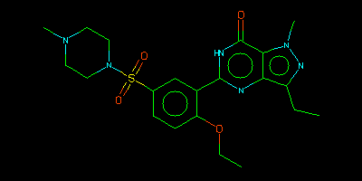
viagra = "CCc1nn(C)c2c(=O)[nH]c(nc12)c3cc(ccc3OCC)S(=O)(=O)N4CCN(C)CC4"
cialis = "CN1CC(=O)N2[C@@H](c3[nH]c4ccccc4c3C[C@@H]2C1=O)c5ccc6OCOc6c5"
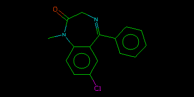
valium = "CN1C(=O)CN=C(c2ccccc2)c3cc(Cl)ccc13"
xanax = "Cc1nnc2CN=C(c3ccccc3)c4cc(Cl)ccc4-n12"

For example,

viagra Carbon labels are generally omitted in renderings.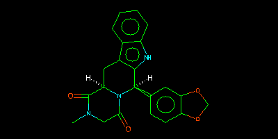

cialis

valium

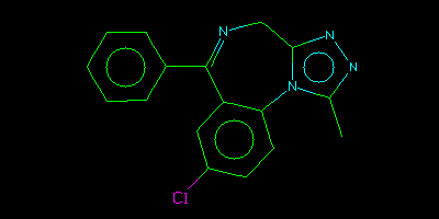xanax (Examples@[daylight].com)

Chemical compounds are of bounded degree. Most small compounds are planar but exceptions are conceivable. Hydrogen atoms can be specified in SMILES but they are usually omitted and, if so, they, and the bonds to them, are left out of the resulting graph.

The information-content routines were "told" that the graphs were of bounded degree, and were given the maximum degree of each element. Apart from that, they were not given any hard-wired chemical information. It is of course possible to include example graphs as background knowledge.

The following table shows the results of experiments on viagra, cialis, valium and xanax [daylight.com], singly and in various combinations.

viagra cialis valium xanax total 267 262 169 194 892 information(.) in bits

 

viagra cialis valium xanax viagra (75) 180 217 211 cialis 168 (55) 160 172 valium 119 108 (48) 86 xanax 128 133 115 (59) information(left|top) in bits (The diagonal elements are small, but not tiny, because there is no great prior expectation of X|X.)

 

viagra cialis|viagra valium|viagra, cialis xanax|viagra, cialis, valium total 267 168 111 88 634 information(.|.) in bits (Note that viagra and cialis are less helpful to valium than cialis alone.)

Summary

The problem of calculating a graph's information content is so general as to be almost insufficiently specified when one considers factors such as but not limited to:

degree:	bounded | unbounded, sparse | dense
(in?)dependence of:	Vertex label, Vertex degree, Edge label, cycle length
label matching:	equal or "close" (perhaps squared difference for continuous?)
subgraph matching:	equal or approximate (even varieties of approximate tree matching are hard)

A prototype algorithm exists for some of the above options "pinned down". It has been used to calculate the information content of graphs derived from small chemical compounds. It takes a few seconds to process compounds containing dozens of elements. Its worst-case time complexity is exponential, but certain speed-up techniques are conceivable, such as,

hash table of small sub-graphs to find good candidate matches quickly, and

halting context matching at a distance threshold.

References

(Added later: Also see L. Allison, 'Coding Ockham's Razor', Springer, 2018, isbn13:978-3319764320, doi:10.1007/978-3-319-76433-7, and [www.cantab.net/users/mmlist/MML/A/].)

Appendix

Examples of graphs, automorphism groups and distinguishable Vertex orderings.

K4  *----*   |A|=4!
    |\  /|
    | \/ |   all 4! Vertex orderings are indistinguishable
    | /\ |
    |/  \|
    *----*

C4  *--*     |A|=8  (4 rotations × reflection)
    |  |
    |  |
    *--*

  4!/8 = 3 distinguishable Vertex orderings
    1--2    1--2    1--3
    |  |    |  |    |  |
    |  |    |  |    |  |
    4--3    3--4    4--2

  and their implied adjacency matrices
    _101    _110    _011
    1_10    1_01    0_11
    01_1    10_1    11_0
    101_    011_    110_

G = *--*    |A|=4   (reflection × reflection)
    |\ |
    | \|
    *--*

  4!/4 = 6 distinguishable Vertex orderings
    1--2    1--2    1--3    2--1    2--1    3--1
    |\ |    |\ |    |\ |    |\ |    |\ |    |\ |
    | \|    | \|    | \|    | \|    | \|    | \|
    4--3    3--4    4--2    4--3    3--4    2--4

G = W--B
    |  |
    |  |
    B--W